Recurrent Neural Network

1. Local dependency assumption: The sequential information of all previous timestamps can be encoded into one hidden representation. 2-order Markov assumption. Temporal receptive field: 2 $\begin{array}{l}{P\left(x_{1}, \ldots, x_{T}\right)} \\ {=\prod_{t=1}^{T=1} P\left(x_{t} | x_{1} \ldots, x_{t-1}\right)} \\ {=\prod_{t=1}^{T} g\left(s_{t-2}\right] x_{t-1} )}\end{array}$

2. Parameter Sharing assumption: If a feature is useful at time $t_1$, then it should also be useful for all timestamp $t_2$ $\begin{array}{l}{P\left(x_{t_{1}+\tau}, \ldots, x_{t_{n}+\tau}\right)} \\ {=P\left(x_{t_{1}}, \ldots, x_{t_{n}}\right)}\end{array}$

但是实际上，两个假设在实际问题上都不会成立

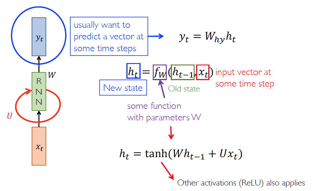
$h_t$ is used to encode the information from all past timesteps

Stationary assumption

we use the same parameters, W and U

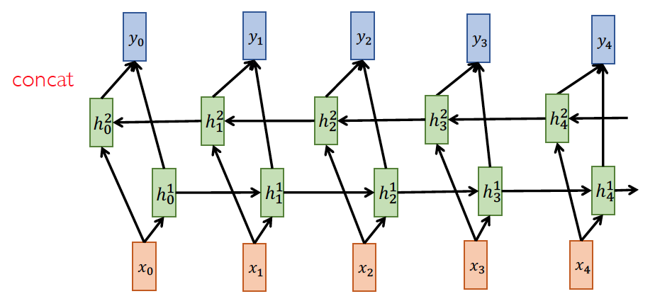
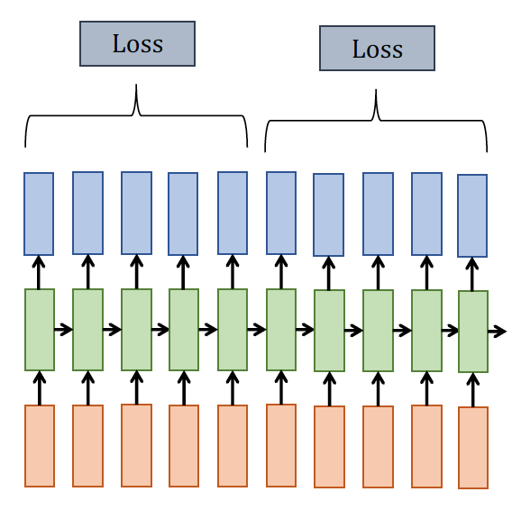
Bidirectional RNN

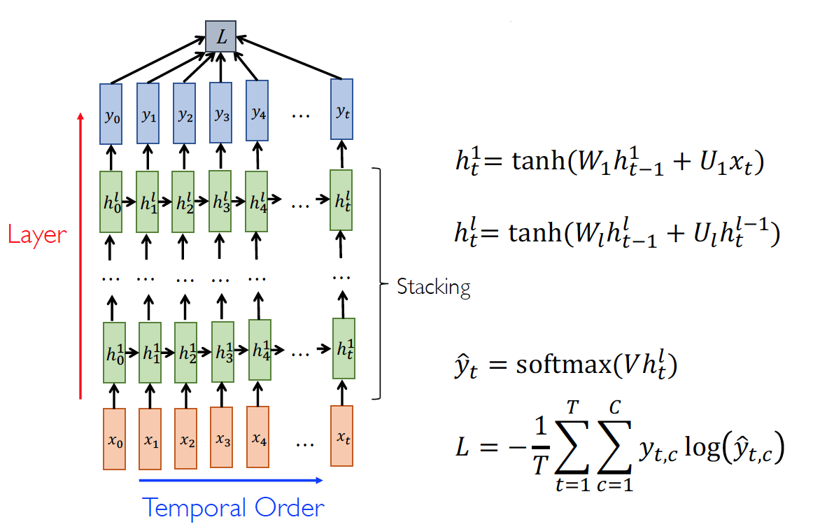
Deep RNN

RNN for LanguageModel(LM)

• Advantages:
  • RNNs can represent unbounded temporal dependencies
  • RNNs encode histories of words into a fixed size hidden vector
  • Parameter size does not grow with the length of dependencies
• Disadvantages:
  • RNNs are hard to learn long range dependecies present in data

Back-Propagation Through Time(BPTT)

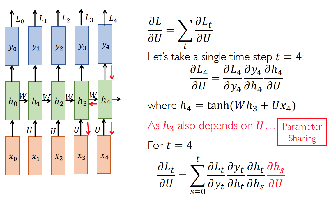$\begin{array}{c}{\frac{\partial L_{t}}{\partial U}=\sum_{s=0}^{t} \frac{\partial L_{t}}{\partial y_{t}} \frac{\partial y_{t}}{\partial h_{t}} \frac{\partial h_{t}}{\partial h_{s}} \frac{\partial h_{s}}{\partial U}} \\ {\frac{\partial h_{t}}{\partial h_{t-1}} \frac{\partial h_{t-1}}{\partial h_{t-2}} \ldots \frac{\partial h_{s+1}}{\partial h_{s}}}\end{array}$ Gets longer and longer as the time gap (t-s) gets bigger!

It has to learn a same transformation for all time steps

Truncated BPTT

原始的 RNN 计算 BPTT

1. Forward through entire sequence to compute loss

2. Backward through entire sequence to compute gradient

$\frac{\partial h_{t}}{\partial h_{t-1}} \frac{\partial h_{t-1}}{\partial h_{t-2}} \dots \frac{\partial h_{s+1}}{\partial h_{s}}$计算代价过高

Truncated BPTT:

Run forward and backward through chunks of the sequence instead of whole sequence

Truncation: carry hidden states forward in time forever, but only back-propagate for some smaller number of steps

Learning Difficulty

Vanishing or Exploding gradient

$$\frac{\partial h_{t}}{\partial h_{s}}=\frac{\partial h_{t}}{\partial h_{t-1}} \frac{\partial h_{t-1}}{\partial h_{t-2}} \dots \frac{\partial h_{s+1}}{\partial h_{s}}$$

where $h_{t}=W f\left(h_{t-1}\right)+U x_{t}$ $\frac{\partial h_{t}}{\partial h_{s}}=\prod_{k=s+1}^{t} W^{\mathrm{T}} \operatorname{diag}\left[f^{\prime}\left(W h_{k-1}\right)\right]$

$$\left\|\frac{\partial h_{t}}{\partial h_{t-1}}\right\| \leq\left\|W^{\mathrm{T}}\right\|\left\|\operatorname{diag}\left[f^{\prime}\left(W h_{t-1}\right)\right]\right\| \leq \sigma_{\max } \gamma$$

• $\sigma_{max}$ is the largest singular value of $W^T$
• $\gamma$ is the upper bound of $\left\|\operatorname{diag}\left[f^{\prime}\left(W h_{t-1}\right)\right]\right\|$

• $\gamma$ depends on activation function $f$, e.g. $$\left

  \tanh ^{\prime}(x)\right

  \leq 1,\left

  \sigma^{\prime}(x)\right

  \leq \frac{1}{4}$$

Conclusion:

• RNNs are particularly unstable due to the repeated multiplication by the same weight matrix
• Gradient can be very small or very large quickly

Vanishing Gradient

为什么梯度消失是个问题？

• 不能学习到 long term dependencies，在语言模型中，在很远的词是不会影响到下一个词的预测的

对于梯度消失的小 trick：

• Orthogonal Initialization（正交初始化）：
  • 将参数 W 初始化为一个random orthogonal matrix (i.e. $W^{\mathrm{T}} W=W W^{\mathrm{T}}=I$), 所以一直乘$W^T$不会改变norm $\left\|W^{\mathrm{T}}\right\|$，因为 $\left(W^{\mathrm{T}} v\right)^{\mathrm{T}}\left(W^{\mathrm{T}} v\right)=v^{\mathrm{T}} W W^{\mathrm{T}} v=v^{\mathrm{T}} v$
  • Initialize W with small random entries, the $\operatorname{diag}\left[f^{\prime}\left(W h_{t-1}\right)\right] \approx I$

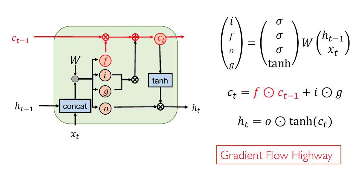
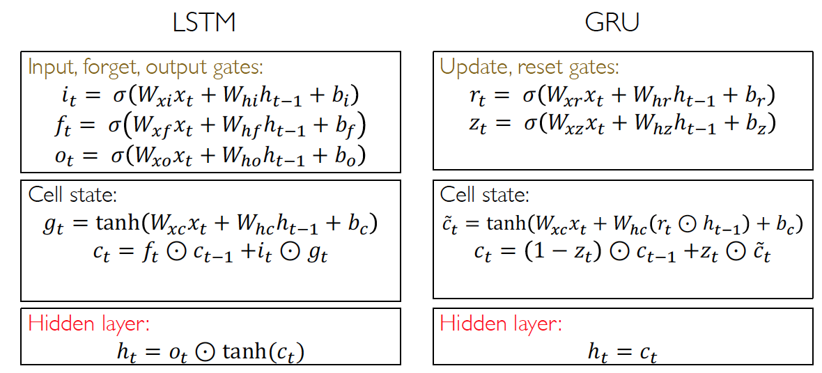
Long Short-Term Memory(LSTM)

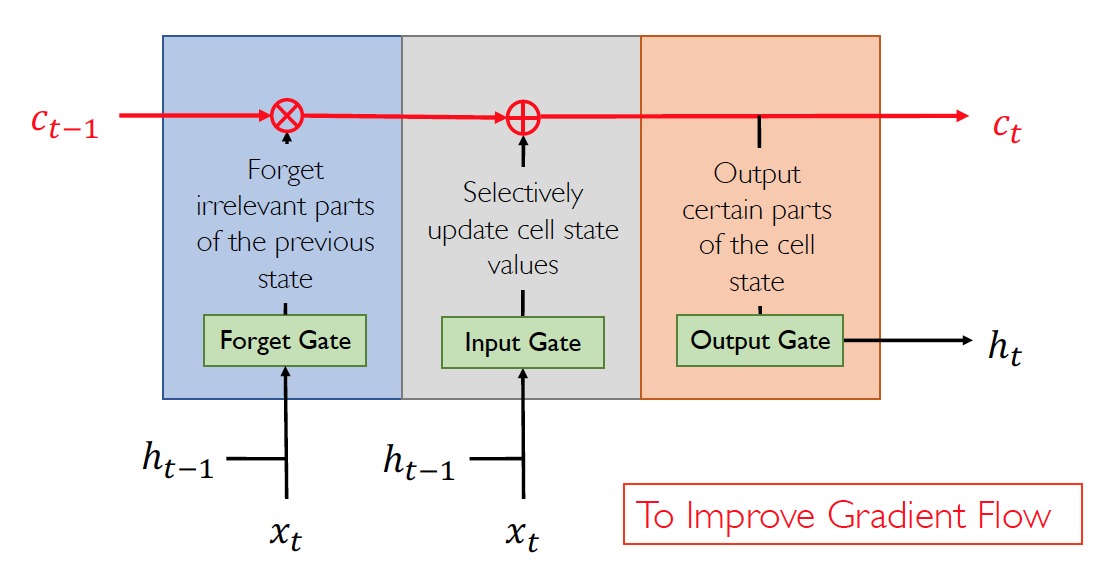
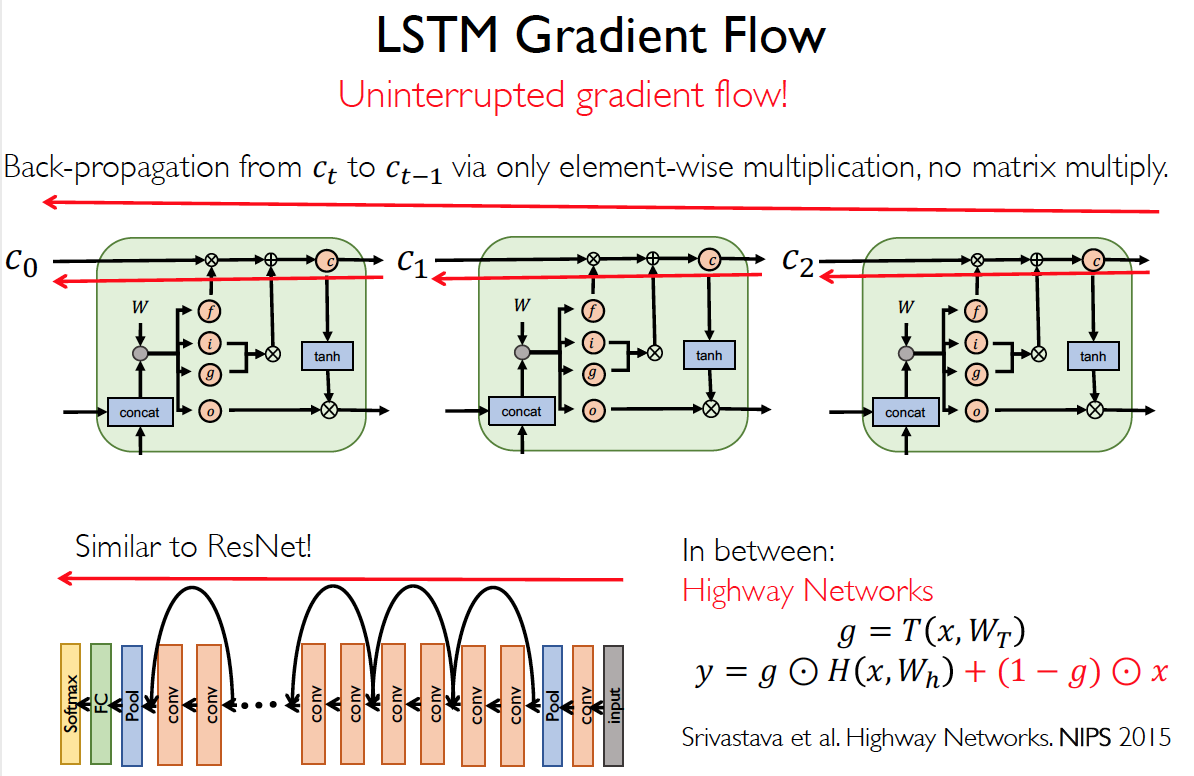$\begin{aligned} c_{t} &=f_{t} \odot c_{t-1}+i_{t} \odot g_{t} \\ &=f_{t} \odot f_{t-1} \odot c_{t-2}+f_{t} \odot i_{t-1} \odot g_{t-1}+i_{t} \odot g_{t} \\ &=\sum_{\tau=0}^{t} f_{\tau} \odot \cdots \odot f_{\tau+1} \odot i_{\tau} \odot g_{\tau} \end{aligned}$ As long as forget gates are open (close to 1), gradients may pass into $g_t$ over long time gaps

• Saturation of forget gates (=1) doesn’t stop gradient flow
• A beeter initialization of forget gate bias is e.g. 1

Add ‘peephole’ connections to the gates

• Vanilla LSTM $\begin{aligned} i_{t} &=\sigma\left(W_{x i} x_{t}+W_{h i} h_{t-1}+b_{i}\right) \\ f_{t} &=\sigma\left(W_{x f} x_{t}+W_{h f} h_{t-1}+b_{f}\right) \\ o_{t} &=\sigma\left(W_{x o} x_{t}+W_{h o} h_{t-1}+b_{o}\right) \end{aligned}$

• Peephole LSTM

$$\begin{aligned} i_{t} &=\sigma\left(W_{x i} x_{t}+W_{h i} h_{t-1}+W_{c i} c_{t-1}+b_{i}\right) \\ f_{t} &=\sigma\left(W_{x f} x_{t}+W_{h f} h_{t-1}+W_{c f} c_{t-1}+b_{f}\right) \\ o_{t} &=\sigma\left(W_{x 0} x_{t}+W_{h o} h_{t-1}+W_{c o} c_{t}+b_{o}\right) \end{aligned}$$

There is no significant performance improvement by peephole

None of the variants can improve upon the standard LSTM significantly

The forget gate and the output activation function (if cell state unbounded) to be its most critical components

Thus, we can couple the input and forget input ($f_{t}=1-i_{t}$) to work well->GRU

Gated Recurrent Unit(GRU)

GRU and LSTM yield similar accuracy, but GRU converges faster than LSTM

Exploding Gradient

L1 or L2 penalty on Recurrent Weight:

Regularize W to ensure that spectral radius of W not exceed I: $\|W\|_{2} \leq I$

对于梯度爆炸的小 trick：

• Gradient Clipping: if $\|\hat{\mathbf{g}}\| \geq \text { threshold }$ , $\hat{\mathbf{g}} \leftarrow \frac{\text {threshold}}{\|\hat{\mathbf{g}}\|} \hat{\mathbf{g}}$

What if Batch Normalization?

batch normalization (makes the optimization landscape much easier to navigate and smooth the gradients!) $\overline{a}_{i}^{l}=\frac{g_{i}^{l}}{\sigma_{i}^{l}}\left(a_{i}^{l}-\mu_{i}^{l}\right)$

$$\mu_{i}^{l}=E_{x \sim P(x)}\left[a_{i}^{l}\right]$$ $$\sigma_{i}^{l}=\sqrt{E_{x \sim P(x)}\left[\left(a_{i}^{l}-\mu_{i}^{l}\right)^{2}\right]}$$

Problems when applied to RNNs:

• Saturation of forget gates(=1) doesn’t stop gradient flow
• Needs different statistics for different time-steps
  • problematic if a test sequence longer than any training sequences
• Needs a large batch size
  • problematic as RNNs usually have small batches (recurrent structures, e.g.LSTM, usually require larger memory usage )

Layer Normalization

$$\boldsymbol{h}^{t}=f\left[\frac{\boldsymbol{g}}{\sigma^{t}} \odot\left(\boldsymbol{a}^{t}-\mu^{t}\right)+\boldsymbol{b}\right]$$ $$\mu^{t}=\frac{1}{C} \sum_{i=1}^{C} a_{i}^{t}$$ $$\sigma^{t}=\sqrt{\frac{1}{C} \sum_{i=1}^{C}\left(a_{i}^{t}-\mu^{t}\right)^{2}}$$

• g(gain) and b(bias) are shared over all time-steps, the statistics are computed across each feature and are independent of batch sizes
• After multiplying inputs and state by weights but right before nonlinearity

Weight Normalization

• Lower computational complexity and less memory usage much faster then BN
• Prevents noise from the data without relying on training data

Practical Training Strategies

• Mismatch in training and inference
• curriculum learning
• scheduled sampling
• variational dropout