CNN

Convolutional Neural Network

学习 feature 的层次化表达

Convolution

连续函数： $(f * g)(t)=\int_{-\infty}^{\infty} f(\tau) g(t-\tau) \mathrm{d} \tau$ 离散函数： $(f * g)[n]=\sum_{m=-\infty}^{\infty} f(m) g[n-m]$

Cross-Correlation

Cross-correlation, sliding inner product

是用来看两个序列$f(\tau), g(\tau)$ 相似度测量的一个指标

$$(f * g)(\tau)=\int_{-\infty}^{\infty}\overline{ f(t) }g(t+\tau) \mathrm{d} t$$

Convolution vs. Cross-Correlation

cross-correlation 的函数 f(t)和 g(t)等价于 convolution 的函数 $\overline{f(-t)}$ 和 g(t) $[f(t) \star g(t)](t)=[\overline{f(-t)} * g(t)](t)$ 在 CNN 里面使用更直观的 cross-correlation 的操作

Notation

Volume/Tensor：height * width * depth/channels

Kernel/Filter

Local Connectivity

Locality Assumption：local information is enough for recognition

每个 patch（local region of the input volume）会连接到一个neuron

每个 patch 就是一个感知野（Receptive field） $S(w, h, d')=(I * K)(w, h, d')=\sum_{d} \sum_{i} \sum_{j} I(w+i, h+j, d) K(i, j, d)$ I 是 Input volume，K 是 kernel, 输出的 S(w, h)是一个neuron，是 filter K 和input 的小 chunk I(w+i, h+j)的点积 $(f \star g)[n] \triangleq \sum_{m=-\infty}^{\infty} \overline{f[m]} g[m+n]$ 使用了 cross-correlation

Parameter Sharing

Translation Invariance Assumption: If a feature is useful at spatial position (x, y), then it should also be useful for all positions (x’, y’)

不同的空间位置，共享相同的 sliding window 的权重。

Filter 如果是 $5*5*3$ 参数值：$5*5*3+1(bias)$

Strid: 1

Padding: ‘Valid’

最后输出feature map

注意：实际上没有 sliding 这个动作，是在每个位置（w, h）上加一个 neuron

叠加多个 kernel，增加 feature map 的深度

Dilated Convolution

空洞卷积：Fisher Yu, Vladlen Koltun. “Multi-Scale Context Aggregation by Dilated Convolutions.” ICLR, 2016.

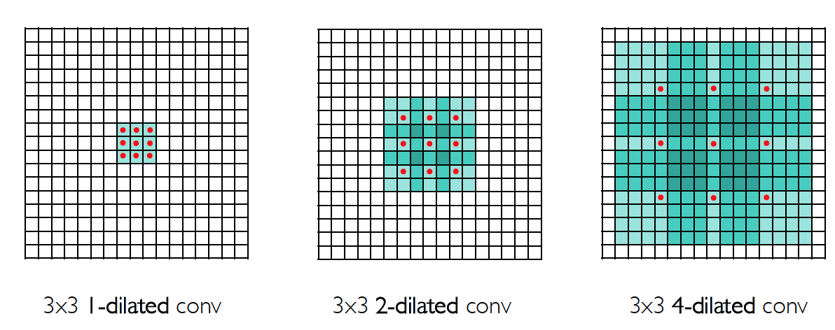
空洞卷积的优点：support exponential expansion of the receptive field without loss of resolution or coverage

Stride

步幅：如果想要 subsample output，可以增加stride $\begin{array}{l}{\text { height }_{\text{new}}=\lceil\text { (height-filter }+ 1) / \text { stride } \rceil+1} \\ {\text { width }_{\text { new }}=\lceil(\text { width-filter }+1) / \text { stride }\rceil+ 1}\end{array}$

Padding

填充：在原来的 map 外面，增加 n 圈 0 $\begin{array}{l}{\text { height }_{\text { new }}=\left\lceil\text { (height-filter }+ 2^{*} \text { pad) } / \text { stride }\right\rceil} \\ {\text { width }_{\text { new }}=\left\lceil(\text { width-filter }+2^{*} \text { pad }\right) / \text { stride } \rceil}\end{array}$ 经过多层的 convolutions，减小了 spatial size W*H，而且在 boundary 的信息是有效的，使用 padding 能够减轻这个问题。

Activation Function

ReLU

max(0, x)

Leaky ReLU

max(0.1x, x)

优点：

• 在正的区域（>0），不会饱和 saturate
• 计算很高效
• 收敛速度比 sigmoid、tanh快（比如快 6 倍）
• 在生物上比 sigmoid 更有解释力，说服力

缺点：

• 不是以 0 为中心的对称
• an annoyance->Leaky ReLu

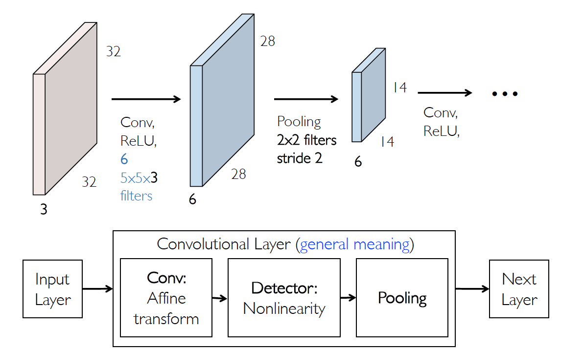
Convolutional Layer

在空间维度上收缩的太快不好，效果不好

• an input volume of size: $W1*H1*D1$

• hyperparameters:

  • filters 的数量：D2(也是下一层的 depth)
  • kernel size：K
  • Stride：S
  • padding：P

• an output volume of size $W2*H2*D2$ $\begin{array}{l}{W_{2}=\left(W_{1}-K+2 P\right) / S+1} \\ {H_{2}=\left(H_{1}-K+2 P\right) / S+1}\end{array}$

• 因为 parameter sharing，参数数量：$(K*K*D1+1)*D2$

Pooling

池化：

• 缓解 convolutional layer 对 location 过度sensitivity，即提高 translation invariance
• 在处理过程中也可以减低维度

池化的操作对于每个 activation map 都是独立的。

池化只是降低 width 和 height 的维度，depth 在池化前后保持不变

max pooling

最大池化

average pooling

平均池化

spatial pyramid pooling

空间金字塔池化，缓解 multiscale 的问题

用不同 scale 的pooling，然后再 concat 起来，生成一个定长的表达

Convolutional Network：Typical Layer

LeNet

AlexNet

Backpropagation Algorithm

Weight Initialization

如果 weight 初始化 W=0，这个网络压根就不能学习

如果 weight 从一个正态分布采样（均值=0，方差=0.4），收敛速度太慢

如果 weight 从一个正态分布采样（均值=0，方差和$\sqrt{2/n_i}$）成正比

Xavier Initialization

$$\mathbb{E}\left[x_{j}\right]=0, \mathbb{E}\left[x_{j}^{2}\right]=\gamma$$ $$h_{i}=\sum_{j=1}^{n_{\mathrm{in}}} W_{i j} x_{j}$$ $$\begin{array}{c}{\mathbb{E}\left[h_{i}\right]=\sum_{j=1}^{n_{\mathrm{in}}} \mathbb{E}\left[W_{i j} x_{j}\right]=0} \\ {\mathbb{E}\left[h_{i}^{2}\right]=\sum_{j=1}^{n_{\mathrm{in}}} \mathbb{E}\left[W_{i j}^{2}\right] \mathbb{E}\left[x_{j}^{2}\right]=n_{\mathrm{in}} \sigma^{2} \gamma^{2}}\end{array}$$ $$\sigma^{2}=1 / n_{\mathrm{in}}$$

He Initialization

$$\sigma^{2}=2 / n_{\mathrm{in}}$$

合适的 Initialization，可以避免signals指数级的增大或者减小

Batch Normalization

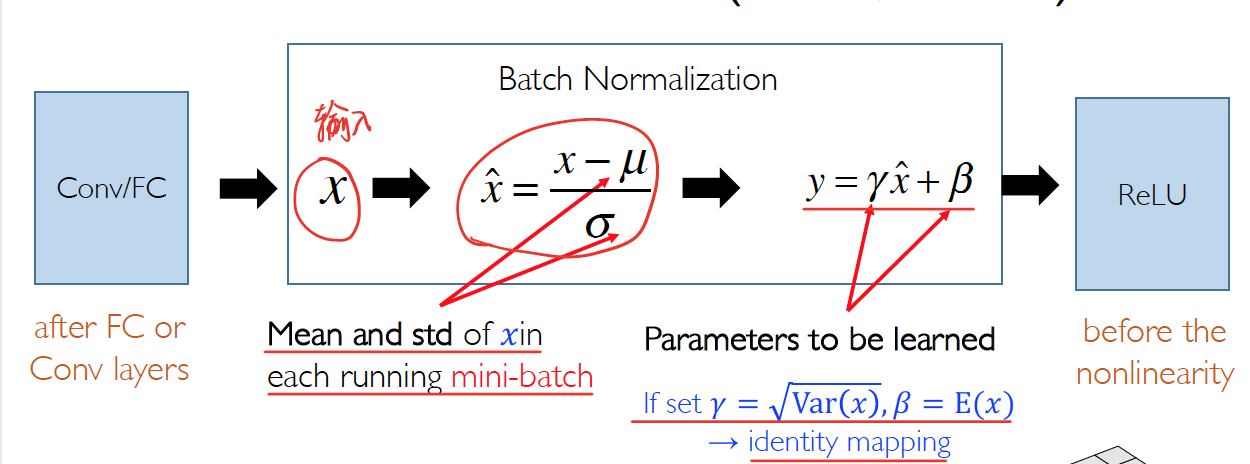
在 mini-batch 的 examples 中做 normalize

mini-batch size：n

feature maps size: w*h

所以有$n*w*h$个元素会一起 normalized，每个 feature map 都有一对$\gamma, \beta$

这个是对每个 channel 做的normalized

加了 batch normalization 能够有更大的learning rate，产生更高的 test accuracy

• 没有 BN，每层的值很快就达到饱和
• 有 BN，尽管前面的层相对比较饱和，但是因为下一层做了 BN 就会到一个 effective unsaturation 的状态

为什么要 BN？

Covariate shift

输入层的输入分布在 training 过程中会改变

internal covariate shift(ICS)

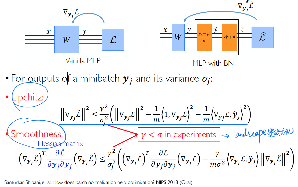
The “smoothing” effect of BN makes the optimization landscape much easier to navigate

因为一个 small batch 会导致一个 batch 的 statistics 错误的估计（减小 BN batch size ，会导致模型错误率大幅度上升），所以就引申出来了不同的 normalization 的方法

• Batch Norm
• Layer Norm
• Instance Norm
• Group Norm，在不同 batch size 的情况下，准确率很稳定

Invariance & Equivariance

不变性和等变性

• equivariance：An Operator f is equivariant with respect to a Transformation T when the effect of T is detectable in the Output of f:

$$f(T(x))=T(f(x))$$

• invariance: An Operator f is invariant with respect to a Transformation T when

  the effect of T is not detectable in the Output of f: $f(T(x))=f(x)$

CNN 通过增加 pooling 层来使得对 small change 有 invariant

但是 CNN 本质上是受限于大量未知的 transformation 的

所以通过数据增广来解决

可否同时保证 equivariance 和 invariance

Capsule

Standard CNN

• AlexNet(8 layers)

• ZFNet(8 layers)

• VGG(19 layers)

• Network in Network(NIN)：
  • convolutions and pooling reduce resolution
    • reduce resolution progressively
    • increase number of channels by 1x1 conv
  • global average pooling in the end
• Inception-v1（GoogLeNet, 22 layers）: 比 AlexNet 的参数小 12 倍，更深的网络却有更少的参数
  • stem Network
  • Stacked Inception Modules:
    • use 1x1 conv to reduce feature maps
  • Classifier output
• Inception-v2
  • add batch normalization: accelerating DNN training, smooth landscape, smooth Lipchitz, Hessian
  • 5x5-> 3x3+3x3: Keep the same receptive field using deeper network with smaller filters
• Inception-v3
  • Convolution Factorization: nxn-> 1xn+nx1 faster training, deeper network
  • Larger input size: 224x224->299x299
• ResNet(152 layers): Residual Network：

1x1 Convolution

使 channels 改变(增加或减少都行），但是不改变 width 和 height

shrinking too fast in the spatial dimensions is not good, doesn’t work well

Highway Networks

$$y=H\left(x, W_{H}\right) \cdot T\left(x, W_{T}\right)+x \cdot C\left(x, W_{C}\right)$$

T: transform gate ，$T(x)=\sigma\left(W_{T}^{T} x+b_{T}\right)$

C: carry gate， 简单的就是$\left(1-T\left(x, W_{T}\right)\right)$

可以让无阻碍的信息流在 information highway 上穿过很多层

Residual Network

当不断 stacking deeper layer 时，56 层 model 在 training 和 test 上都表现的很差，但是不是因为 overfitting，是因为 deepermodel 更难优化，是优化问题

堆叠 residual block, 每个 residual block 有两个 3 x3 的 conv layer，在开始的地方有另一个 conv layer,在结束的地方有 global average pooling

Improving ResNet

1. 和 gooLeNet 相似，使用 bottleneck layer 提高效率，创造更加直接的通路，增加 BN
2. ResNeXt：用多并行的 pathway 增加residual block 的宽度，有点像 inception module

DenseNet

优点：

1. strong gradient flow->deep supervision
2. parameter& computational efficiency, but dimension explosion
3. enables te reuse of low-level features

pooling reduces features map sizes

feature map sizes match within each block

Light-Weight CNN

因为在一些嵌入式系统里面，资源是有限的，需要限制模型的大小，所以要进行模型压缩

1. Netwrok Compression
   1. Pruning
   2. Quantization and Encoding

SqueezeNet

fire modules consisting of a squeeze layer with 1x1 filters feeding into an expand layer with 1x1 and 3x3 filters

效果惊人，在 ImageNet达到 AlexNet 的精度，但是少 50x 的参数，模型大小比 AlexNet 小 510x

Group Convolution

Group convolutions是在 AlexNet 被第一次提出来，将 feature 进行分组，主要是想要降低计算复杂度

Depthwise Separable Convolution

A spatial convolution performed independently over each channel of an input

Depthwise convolution makes each channel highly independent.

How to fuse them together? 1x1 convolution(change #channels)

MobileNet

ShuffleNet

###

Graph Convolution

$$\mathbf{h}_{i}^{(l+1)}=\sigma\left(\mathbf{h}_{i}^{(l)} \mathbf{W}_{0}^{(l)}+\sum_{j \in \mathcal{N}_{i}} \frac{1}{c_{i j}} \mathbf{h}_{j}^{(l)} \mathbf{W}_{1}^{(l)}\right)$$

• $\mathbf{W}_{1}^{(l)}$ weight sharing over all locations
• invariance to permutations
• linear complexity O(E)

Pass messages between nodes to capture the dependence over graphs

AutoML

Neural Architecture Search(NAS)

Learning to learn: Learning the hyper-parameters of a learner

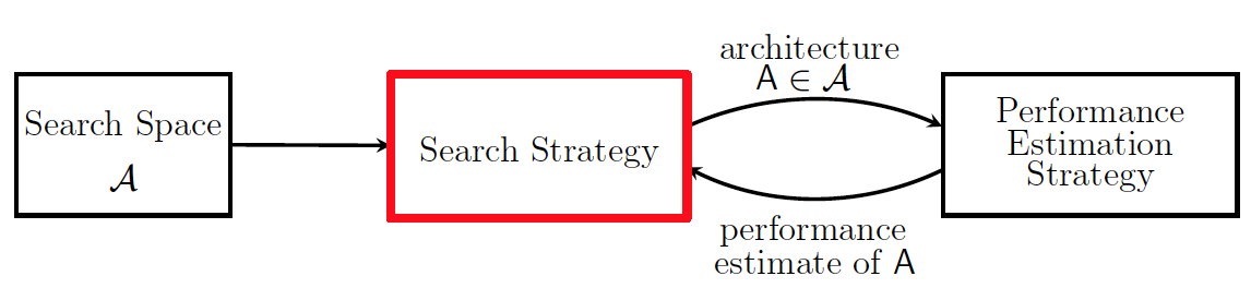
Neural Architecture Search: specify structure and connectivity of a network

• Search Space A: defines which architectures can be represented
• Search Strategy: details fo how to explore the search space
  • Exploration-expoitation trade-off (reinforcement learning)
  • Bayesian optimization
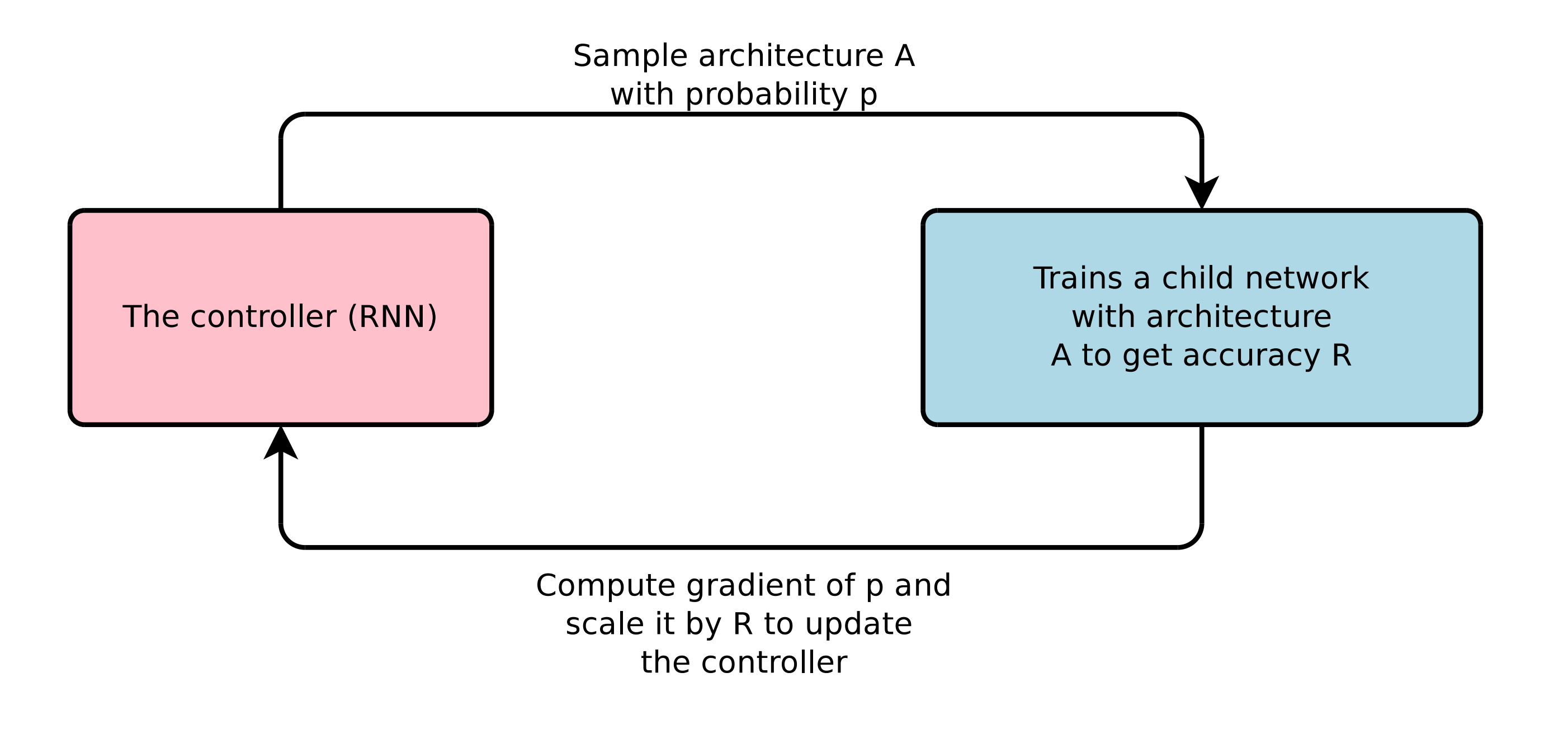
  • At each step, the controller samples a brand new network$A \in \mathcal{A}$
  • Update RNN controller $\theta_c$ based on the accuracy of the child network
• Performance Estimation Strategy: Refers to the process of estimating the predictive performance of an architecture A’ ∈A on unseen data

Reinforcement Learning to optimize the controller

• Reward: Accuracy R

• Action: Hyper-parameters the controller RNN predicts, $a_{1:T}$

• Maximum expected reward: $J\left(\theta_{c}\right)=\mathbb{E}_{P\left(a_{1} ; T ; \theta_{c}\right)}[R]$

• Non-differentiable: supervised learning does not work

• Policy Gradient(Reinforce algorithm)

  • $$\nabla_{\theta_{c}} J\left(\theta_{c}\right)=\frac{1}{m} \sum_{k=1}^{m} \sum_{t=1}^{T}\left[\nabla_{\theta_{c}} P\left(a_{t} \| a_{(t-1) : 1} ; \theta_{c}\right)\left(R_{k}-b\right)\right]$$